

Monopolistic competition is that sub-category of imperfect competition which is nearest to pure competition. It is a market structure in which there are many sellers of a commodity but the product of such seller differs from that of the other sellers.
Thus, in monopolistic competition product are not identical as in perfect competition the products of various producers are close substitutes. Each seller has a monopoly of his own but at the same time he has to face stiff competition from his competition selling close substitutes of his product.
Examples of monopoly competition can be given from the Indian economy there are various manufacturers of soap which produce different brands such as Hamam, Lux, Rexona, Pears, Jai, etc. Thus the manufacturer of Lux has a monopoly of producing it but he has to face competition from the manufacturers of other brands of soap.
Profit Maximisation or Equilibrium under monopolistic Condition
In the situation of monopolistic competition, each competitive firm has partial control over the price of its product, as indicated by the negative slope of its demand curve (AR curve). Each monopolistically firm of a differentiated product behaves so as to get maximum profit.
Determination of equilibrium of a monopolistic competitive firm follows the same general rule of profit maximisation that we have illustrated in the context of perfectly competitive firm. To repeat the equilibrium condition, is determined at the level of output where a firm’s
(i) MR =MC and
(ii) MC curve cuts from below
It may be stated that Chamberlin did not use MC and MR curves, but they are implicit in his analysis.
Study of firm’s equilibrium under monopolistic competition is attempted with reference to two different time periods (i) short period and
(ii) Long period.
-
Short period Equilibrium in Monopolistic Competition
In the short-run a monopolistic competitive firm’s equilibrium is established at the level of output where its MC =MC, and MC is rising, at this level of output
Short period equilibrium does not mean the same price for all firms. Uniforming in price cannot be expected because the products of various firms are not identical cost of production of firms also varies. Normally the average cost (AC) of a large firm is less whereas it is high for small sized firms. Therefore, it is likely that supernorm profits for some firm normal profits for some others and loss to remaining firm would accrue. Thus, a monopolistic competitive firm in the short-run may
- Earn super normal profits i.e., AR>AC
- Earn normal profits ,i.e., AR= AC
- Incur losses, i.e., AR<AC
The three situations for a monopolistic firm are illustrated with the help of following figures
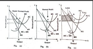
In the all three panels, equilibrium output is determined at point E (where MR= MC and MC is rising.) corresponding to this equilibrium point, equilibrium level of output is OM which is sold at OP price per unit.
Super Normal profit: In Figure (a) OM output is produced at MB cost per unit while it is sold at AM price firm earns a profit of AB per unit. Total profit earned by the equal the shaded area ABCP.
Normal profit: In fig (b) OM output is produced at MB cost per unit and is sold at AM price. The price of the equilibrium output is AM (=OP) and AC is also AM (=OP). It is so because AR curve at point A. Hence, at the level of equilibrium output AR is equal to AC and the firm earns normal profit.
Minimum Loss: In fig (c) OM output is produced at MN cost per unit, but it is sold at OP (=AM) price per unit. The firm incurs a loss equivalent to NM-AM= AN per unit and the total loss of the firm will be NAPC, the shaded area.
Single price of equilibrium output OM is equal to AVC(P=AVC) as curve AVC touches curve AR at point A, firm is incurring loss of fixed cost equivalent to AN per unit it will constitute minimum loss to the firm if the firm is obliged to a price lower than OP (or AM) it would prefer to discontinue production.
Conclusion:
- If marginal revenue (MR) is equal to marginal cost (MC) the firm is in equilibrium the firm raises its production to this level.
- If the average revenue (AR) is more than average cost (AC), the firm cnjoys super normal profits.
- If the average revenue (AR) coincides with average cost (AC), the firm earns normal profit.
- If the average revenue (AR) is less than the average cost (AC), the firm suffers loss. However, if the firm is able to fetch a price which covers at least the average variable cost, it will continue to stay in production.
- If the average revenue (AR) slumps below the average variable cost (AVC). The firm will shut down production.
2. Price and output Determination in the Long period (or Group Equilibrium)
In case of perfect competition, all the firms that were producing the homogeneous product constituted the industry in case of monopoly the firm itself was the industry. However, the concept of industry cannot be applied in case of monopolistic competitive Structure. This is because of its most distinguishing feature – differentiation firms under a monopolistically competitive market structure produce differentiated products. The demand curve of the individual firms cannot be added together to obtain the market demand curve. Thus Chamberlin introduced the concept of ‘product Group’. Product Groups include all firms whose products are closely related, i. e., the group consists of many firm whose products are very much similar to one another and have closely interwoven markets.
The basic difficulty faced in describing the group equilibrium is the vast diversity of conditions which exist in respect of many matters between various firm constituting the group. Prof. Chamberlin attempted to overcome these difficulties by making certain simple assumptions – he calls them ‘heroic’ assumptions – with the basic objective of ignoring the diverse conditions surrounding each firm. His assumptions are:
- All firms in the group are producing more or less identical product.
- All firms have equal share of the market-which means that all of them have similar demand curves (similar in elasticity and position).
- All firms have equal efficiency in production and therefore, have similar cost curves; and
- The number of firms in the group is so large that each firm regards itself independent.
The first three assumptions are known as ‘uniformity’ assumptions’ and the last in known as the ‘symmetry assumption. Given these assumptions, it is possible to explain group equilibrium in the long run.
A monopolistically competitive firm will be in long run equilibrium at the output level where marginal cost (MC)equals marginal revenue (MR).In the long run, the firm under monopolistic competition will (i) neither earn super normal profits, (ii) nor incur losses but, (iii) earn only normal profits.
This is explained as follows:
-
Firms will not earn super normal profits:
Monopolistic competition cannot make super profit in the long-run. There is no restriction in monopolistic competition as to the entry or exit of new firms. If the existing firms make super normal profit new firms will enter the industry. When more and more new firms enter the industry the price will fall and it will near the average cost. The entry of new firms will increase production. But the increase in production does not increase sales. The new firms as well as existing reputed firms to compete with the existing reputed firms introduce their product at a lower price. Thus the existing firms are also compelled to reduce the price of their product. New the price tends to equal the average cost. The individual firm will earn only normal profit. Profits are only when average revenue equals average cost.. So the monopolistically competitive firm will be in long-run equilibrium when firms earn only normal profit which forms part of the cost of production.
-
Firms will not incur losses:
A monopolistically competitive firm in the long-run will not incur loss. If the firms incur loss, some firms will leave the industry, thus reducing the total production now the price will again rise sufficiently to cover the average cost of production.
The foregoing analysis makes it clear that in the long-run only normal profits are available to the firm thus a firm under monopolistic competition will be in the long-run equilibrium.
Where, MR= MC. ….(i)
AR (or P) AC …(ii)
If the first condition is not fulfilled the firm cannot maximise its profit constant shift in production will make the equilibrium unstable.
If the second condition is not realised, firms will enter and exit from the market and influence both output and price if both the conditions are fulfilled disturbing cyclical oscillations are kept in check which will help the firm to reach the equilibrium condition.
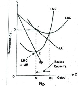
Figure gives long period equilibrium of the firm.
In fig.
- MR =MC and LMC curve is cutting MR curve at point E which is equilibrium point.
- OM is the equilibrium output and PM is the price of equilibrium output.
- At equilibrium output OM, both AR and AC is AM, i.e., AR =LAC. The firm earns only normal profit.
- Long-run equilibrium is not achieved at optimum output OM the difference (MM1) between the actual output (OM₁) and is unused capacity, also known as excess capacity. This is a special feature of monopolistic competition.
Excess capacity: Another interesting fact is noticeable in Fig. At equilibrium point the firm is not making full use of its capacity. In other words, the firms under monopolistic competition have excess capacity because these firms do not produce at the minimum point of its LAS curve it so because negative AR curve is not tangent to U-shaped LAC curve at its minim point.
In perfect competition, AR curve is a horizontal line parallel to X axis as such it touches LAC curve at its minimum point. But under monopolistic competition, AR curve is of negative slope and so touches U-shaped LAC curve at a point which is a bit higher than minimum, i.e., at point A as shown in the figure.
In Fig. optimal level of output (corresponding to the lowest average cost) is OM₁. The equilibrium level is OM. Thus. MM1 represents the excess capacity with the firm which remains unutilised and goes waste.
In short, Excess Capacity=Optimum output – Actual output
MM1=OM1 – OM
Important links
- Dumping- Meaning, Purpose, Price Determination etc.
- Monopoly- Definitions, Features, Classification etc.
- Equilibrium under Discriminating Monopoly
- Price-Discrimination- Degree & Essential Conditions
- Price determination under Oligopoly
- Kinked Demand Curve
Disclaimer: wandofknowledge.com is created only for the purpose of education and knowledge. For any queries, disclaimer is requested to kindly contact us. We assure you we will do our best. We do not support piracy. If in any way it violates the law or there is any problem, please mail us on wandofknowledge539@gmail.com